*Authored by Uber Engineering. Shu-Ming Peng, Jianing He and Ranjib Dey

Introduction

Capacity is a key component of reliability. Uber’s services require enough resources in order to handle daily peak traffic and to support our different kinds of business units. These services are deployed across different cloud platforms and data centers (“zones”). With manual capacity management, it often results in an over-provisioned capacity, which is insufficient for resource usage. Uber built an auto-scaling service, which is able to manage and adjust resources for thousands of micro services. Currently, our auto-scaling service is based on a pure utilization metric. We recently built a new system, Capacity Recommendation Engine (CRE), with a new algorithm that relies on throughput and utilization based scaling with machine learning modeling. The model provides us with the relationship between the golden signal metrics and service capacity. With reactive prediction, CRE helps us to estimate the zonal service capacity based on linear regression modeling and peak traffic estimation. Apart from capacity, the analysis report can also tell us different zonal service characteristics and performance regression. In this article, we will deep dive into CRE’s modeling and system architecture, and present some analysis of its results.

Utilized Metrics

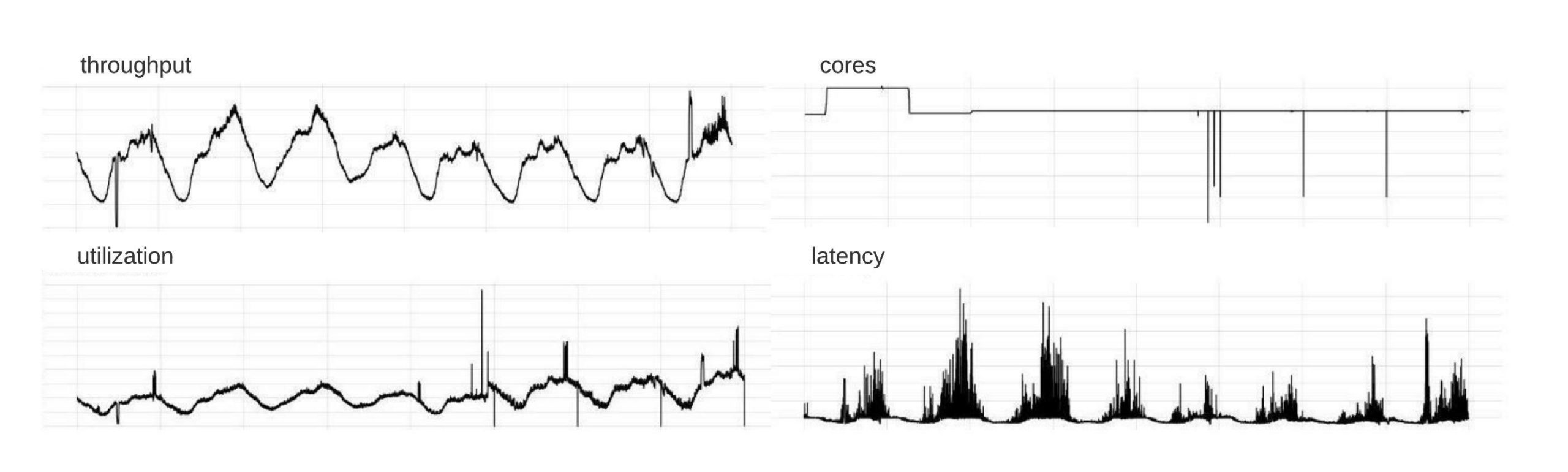
In terms of capacity management, utilization is one of the most widely used metrics for auto-scaling. In CRE, besides utilization, we also consider throughput as another important metric for capacity estimation. Throughput presents the business product requirement. At service level, it translates to requests per second (RPS) for each instance. Whenever there are new products launching and dependencies fan out pattern alterations, it directly results in service throughput changes, which affect the capacity demand. Our goal is to get service capacity or instance counts that meet the utilization requirements. We multiply the number of CPU cores for an instance by the instance count to get total service CPU core allocations. By introducing allocation into the model, we are able to map metrics relationships with service capacity. CRE uses throughput, utilization, and allocation time series data to form a linear regression model. 

CRE Algorithms

In Uber, we have multiple cloud providers. Individually, each of them has various networking stacks, hardware type compositions, and traffic patterns. We mark each zone as an independently scaling target and perform linear regression analysis individually to consider the differences. The performance distinction can be derived from the result and further affect the capacity in the scaling group.

The CRE recommendation process contains several steps, as follows:

1. Peak throughput estimation
2. Define target utilization
3. Linear regression model creation
4. Recommendation generation
5. Guard rails processing

CRE uses peak throughput and target utilization with the metrics relationship generated from step 3 to calculate the capacity instance number. Each stage is critical for the final recommendation and service reliability. In the following sections, we’re going to deep dive into each step.  

Peak Throughput Estimation

Depending on the scaling frequency, which can be hourly, daily, and weekly, the throughput estimation approach that we take can be different. 

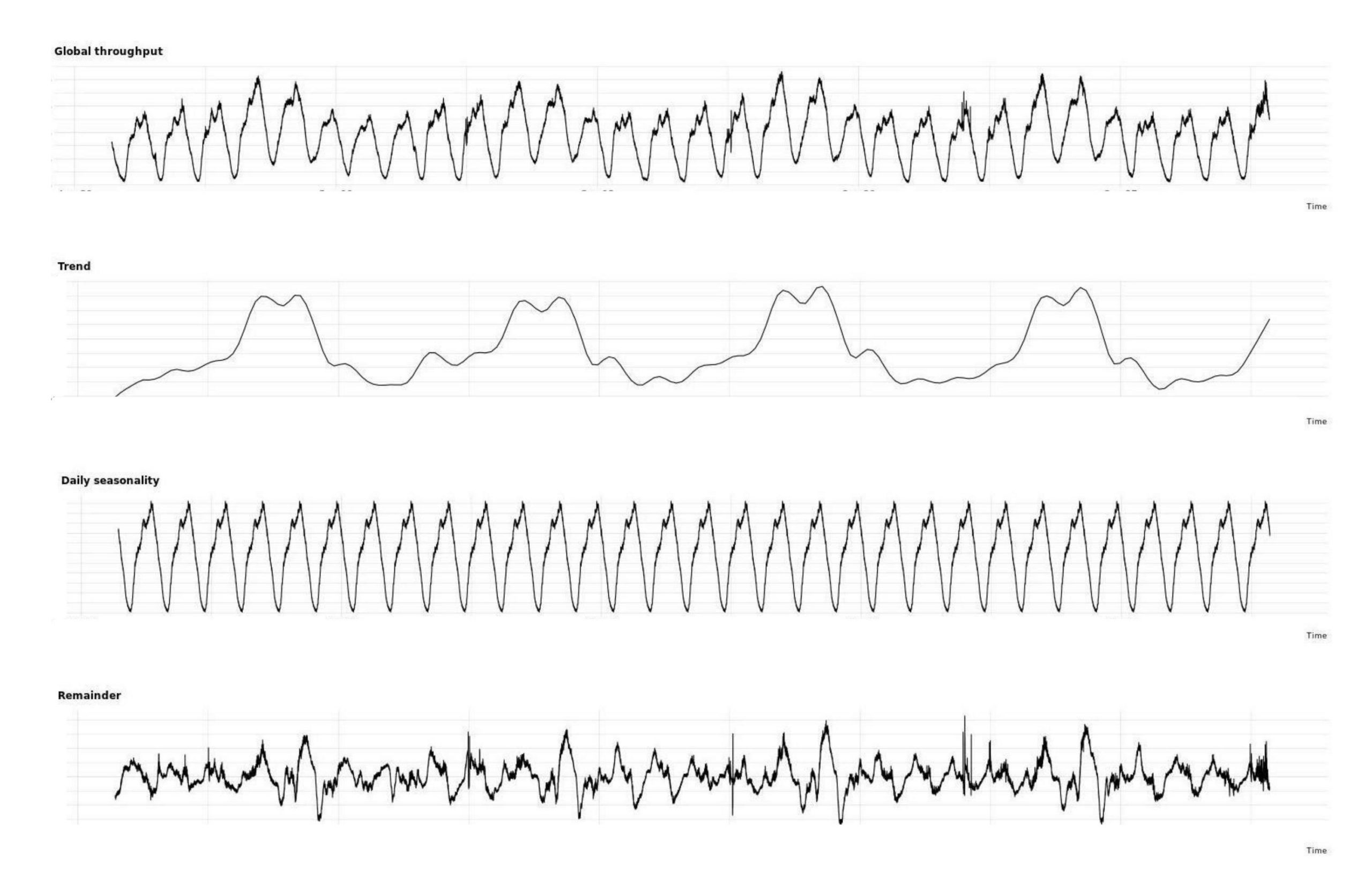
Take throughput estimation for weekly scaling as an example: the target throughput RPS_Target should be the estimation of the next week’s peak traffic. The default throughput estimation method that CRE uses is time series decomposition. The global throughput time series data is then broken down into trend, seasonality, and residue components using the STL-based time series decomposition method. These 3 components additively represent the original global throughput metric. The seasonality component represents a pattern, given a frequency. The trend component represents patterns across days. The example below shows a daily seasonality, with characteristic peaks in US/LatAm commute hours. The residue component is the remainder of the original signal that does not fit in trend or seasonality, generally representing noise. Utilizing the time series decomposition result, CRE is able to provide robust predictions for most services.

Define Target Utilization

Target utilization (Utilization_Target) is the one of the signals required to deduce the capacity number in CRE. The defined signal depicts the estimated future maximum utilization for the service. In order to exploit the resource efficiently, the utilization is defined as high as possible with a reasonable buffer for unforeseen increase. Normal daily traffic should not reach the target utilization. The target utilization should incorporate the usage for incident mitigation. For example, when there is a sudden loss of a zone, traffic will be moved to other zones. The utilization will be higher because of the traffic increase.

Linear Regression: Normalized Throughput and Utilization

For utilization-bound service, utilization, throughput, capacity, service, and hardware performance are common factors, which influence each other. Whenever one of the factors changes, it usually implies that other factors will also be impacted. Since our goal is to estimate service capacity, we need to determine the relationship between the signals. CRE uses utilization and normalized throughput to build a linear regression model. Normalized throughput is deduced by dividing the throughput by the instance core counts—we call it throughput per core (TPC). By normalizing the throughput metric, we are able to reduce factors into utilization and TPC. Performance variation can be observed in the graphs by using the linear regression result’s slope and intercept. The following formula shows the relationship between utilization and TPC:

Utilization =?+? ⨯ TPC

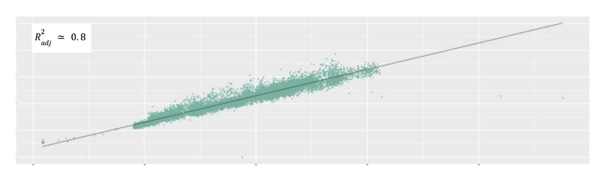
Data has been preprocessed by removing outliers and normalization. If the metric source provides significantly aberrant data points due to control plane issue, the data will be removed during the process. Cross-validation is also used to improve the model quality. When the data is well replicated by the linear regression modeling, it will respond in the adjusted coefficient of determination R²_adj, a statistical measurement corresponding to the outcome quality. As shown in Figure 3, the line well captures the gradient increase tendency of the data, with some outliers. There is a strong linear relationship between the variables. The adjusted coefficient of determination indicates that it succeeds in accurately modeling the data.

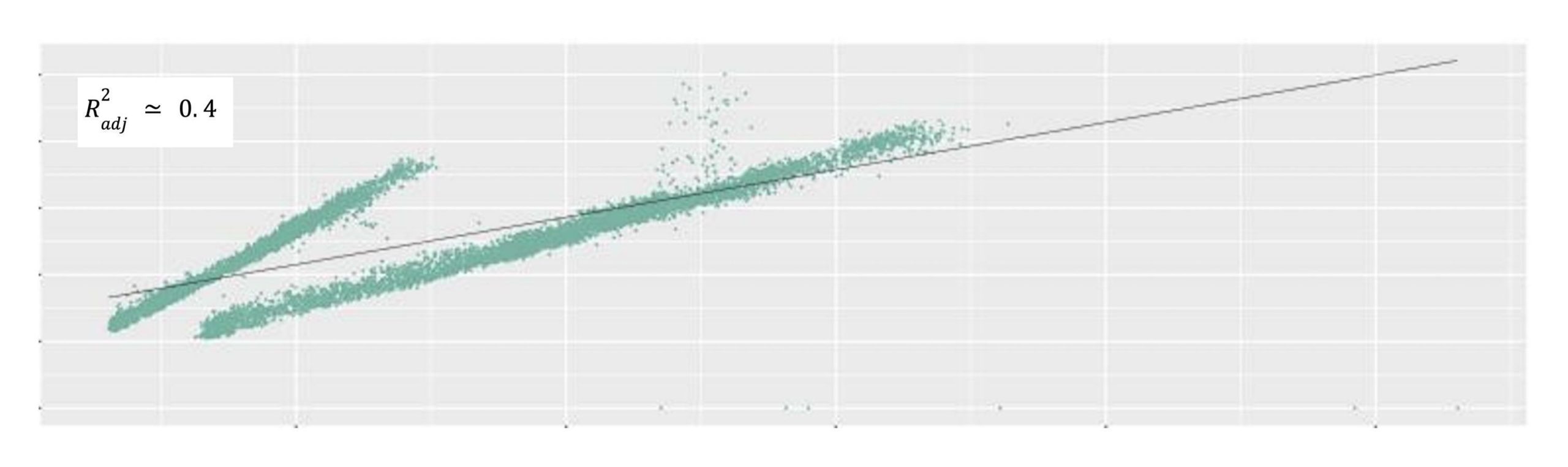
In Figure 4, we can see that the estimated linear relationship does not present the metrics relation. Instead, the data point can be approximately classified as two groups with two distinct linear relationships. This is largely due to diverse service and/or hardware performance over time.  

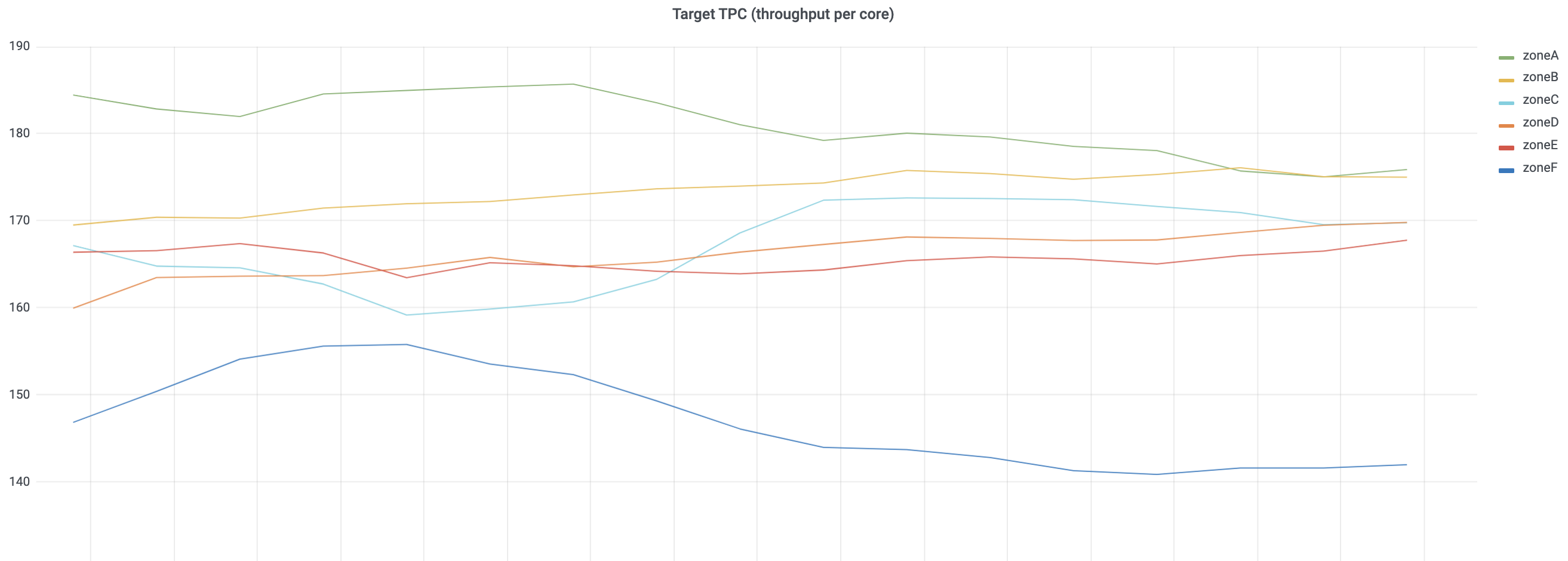
From utilization and the TPC linear relationship function, when we provide a target utilization, the corresponding target TPC can be calculated. For example, we set 0.7 as the target utilization. In Figure 5, the target TPC over time trend shows relatively stable data points. If the adjusted coefficient of determination is stable and reasonable, we can also deduce zonal infrastructure differences from the TPC. Specifically, zoneF has a lower target TPC compared to other zones. The reason might be due to lower infrastructure and hardware efficiency. Also, from the plot, a decreasing trend is observed across zones. Service performance degradation can be a possible factor for further investigation.

Capacity Recommendation Generation

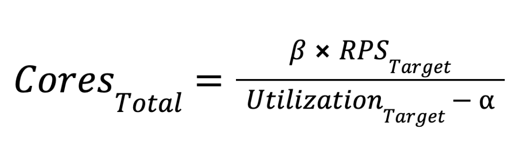
Using the linear regression resulting from ? for utilization intercept and ? for slope, with a predefined target utilization and estimated peak traffic, we are able to calculate the number of cores, which translates to capacity.

Variable Definition:

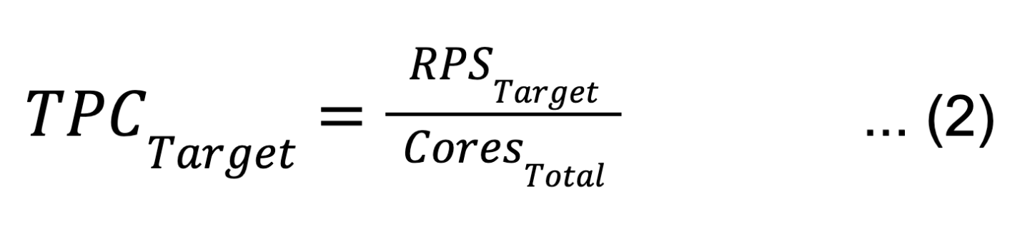
TPC_Target: Target throughput per core (TPC)

RPS_Target: Target RPS provided by peak traffic estimation step

Utilization_Target: Defined target utilization

Cores_Total: Total cores required for the service

Cores_Instance: Number of cores per instance

Formula:

Based on the linear regression model, we update Utilization and TPC to our target value.

The variable definition:

From formulas (1) and (2), we can derive:

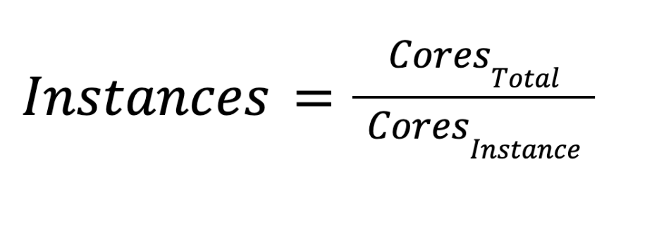
After we get the required total number of cores, we divide it by cores per instance. Finally, we are able to get the recommended capacity instance numbers.

Guard Rail: Result Safeguard

With the capacity recommendation data being generated, in order to safely roll out the changes, we introduce guard rails to inspect the results before auto-scaling. This step is to ensure auto-scaling quality and service reliability. One example guardrail is to check the current capacity against the recommended result. With a predefined percentage threshold, if the recommendation surpasses the percentage of current capacity, guard rail will process the data and adjust the recommendation result accordingly. Other guardrails, like model performance quality, will terminate the auto-scaling process and provide a warning message in the report for engineers to examine the data further.

Architecture

Analysis Flows: Scheduled Analysis

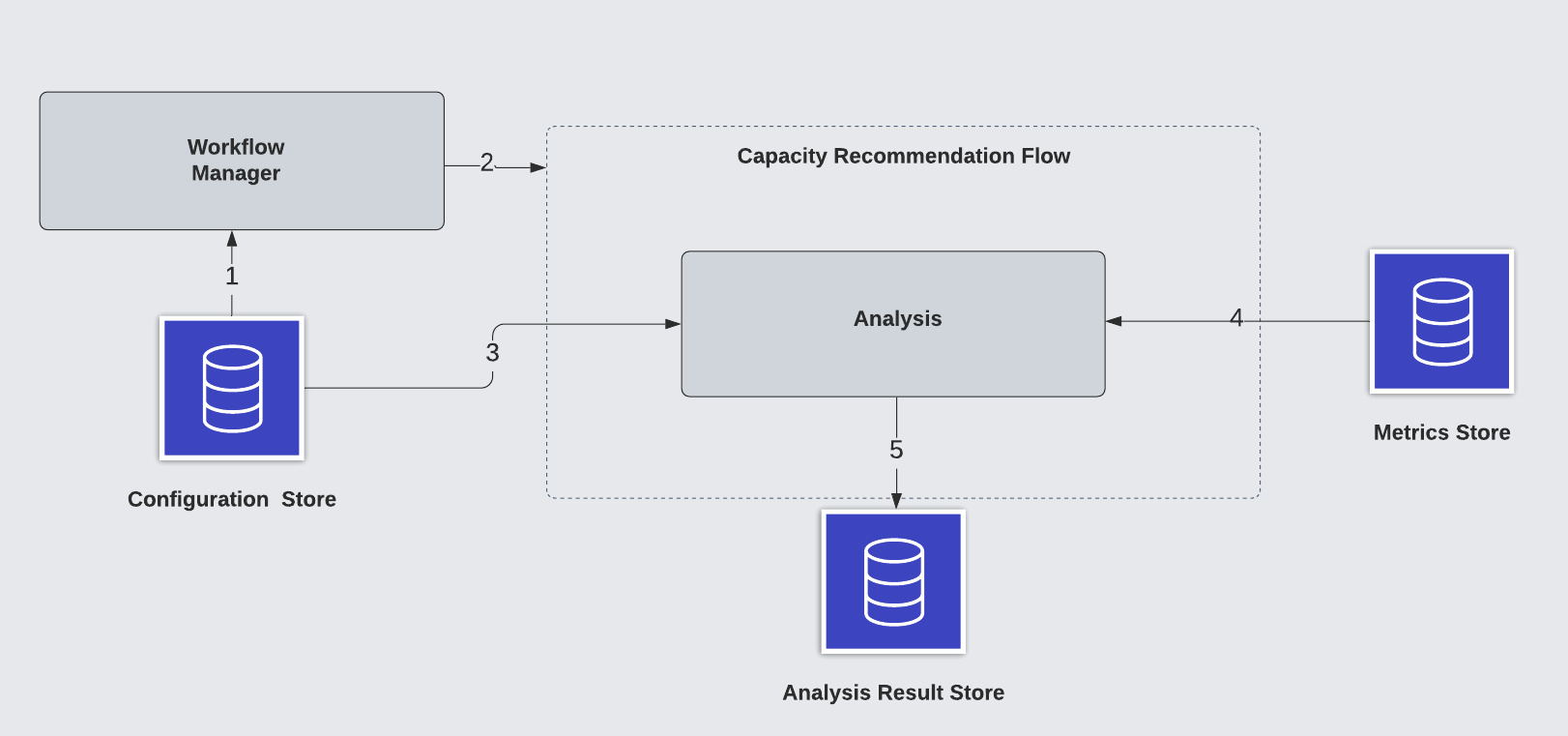
A typical scheduled capacity recommendation flow involves several steps:

1. The workflow manager creates scheduled workflows based on cadence configuration from the configuration store
2. The workflow manager triggers a scheduled workflow
3. With input data gathered from metrics store and data ingestion, the analysis module performs analysis with a selected approach
4. The analysis result is stored in the result store

Analysis Flows: On-Demand Analysis

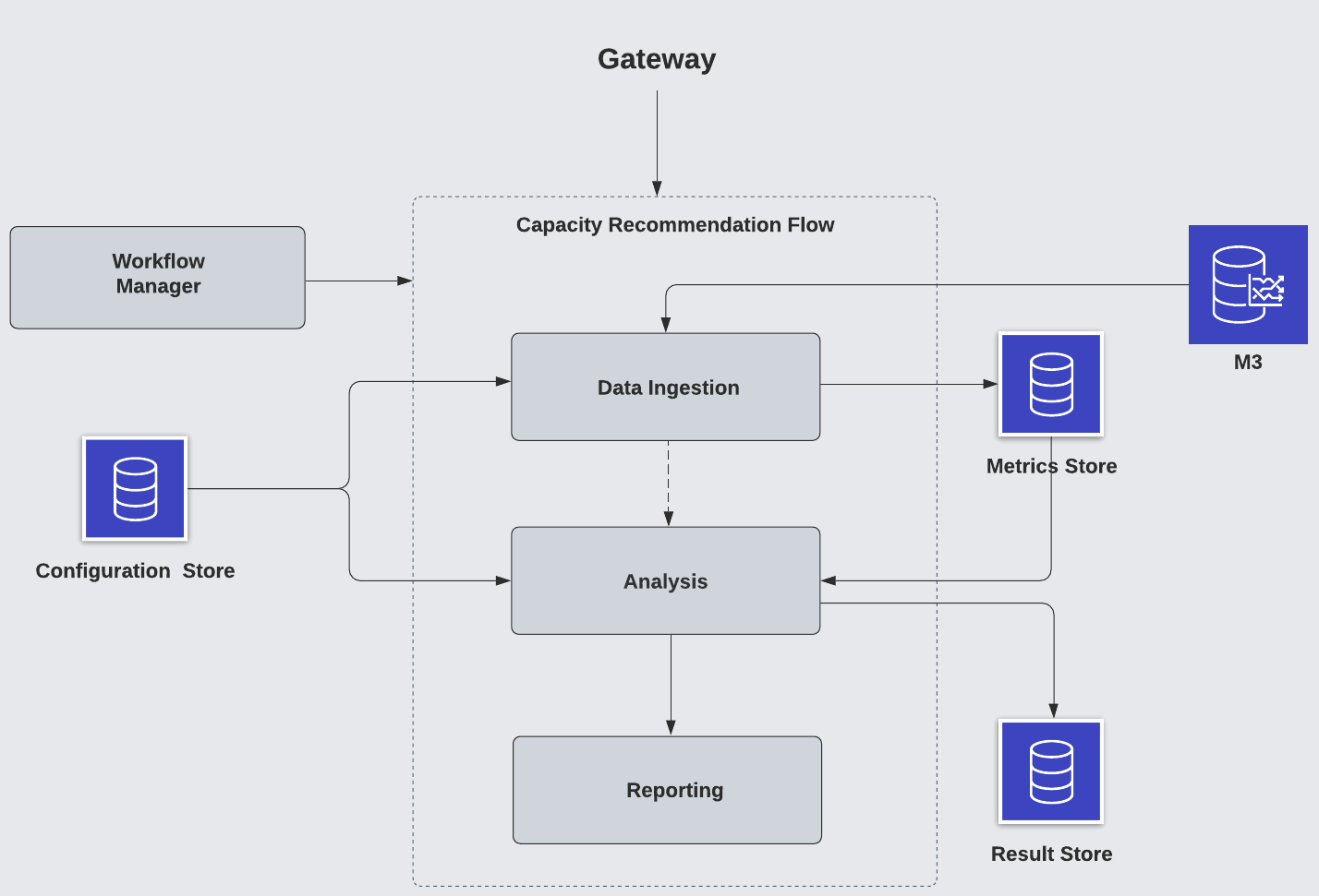
In cases where service owners want to generate capacity recommendations ad hoc, they can utilize the on-demand capacity recommendation flow.

An on-demand capacity recommendation analysis flow is similar to the scheduled flow. The differences are:

1. It is triggered through a user request to the gateway service and the request will be sent to the analysis service where the CRE sat
2. After analyzing and generating the result, an email report will be sent if emails are included in the requests

Data Ingestion Flow

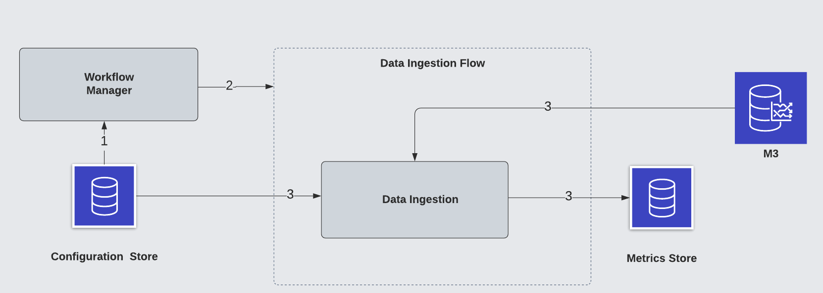
A dedicated data ingestion flow fetches and stores critical services’ raw metric time series data based on configuration. This flow is implemented within a dedicated metric service.

A typical data ingestion flow includes the following steps:

1. The workflow manager creates scheduled workflows based on cadence configuration from the configuration store
2. The workflow manager triggers a scheduled workflow
3. The data ingestion module fetches raw m3 time series data and stores it in the metric store

Result

We have onboarded multiple mission-critical services to the system. The following graphs are one of the service’s scaling results over time. The number of instances scaled up and down according to the analysis result for the period. Figure 8 shows 2 region capacity instances over time. Different services’ build performance, traffic patterns, and underlying hardware performance all contribute to the utilization and linear regression model changes. This leads to various scaling tendencies over time.

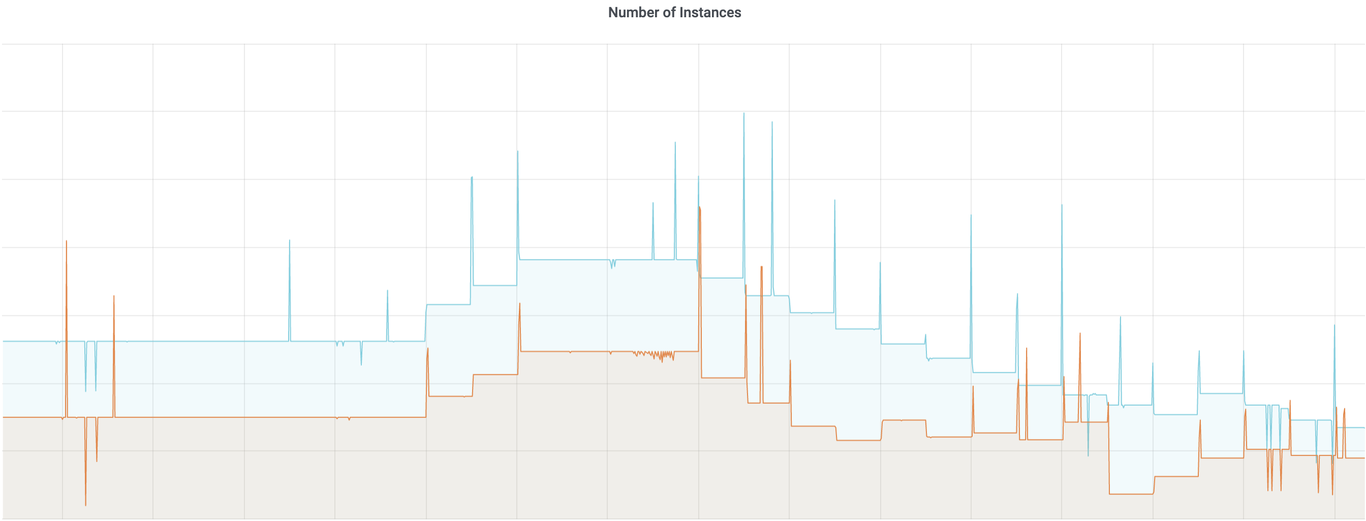
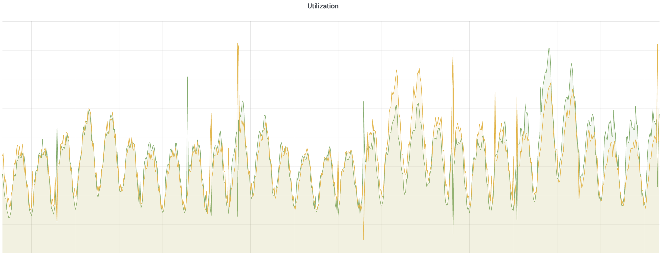
Figure 9 is the scaling service utilization time series, which shows an overall increasing trend. Daily and weekly traffic patterns result in different utilization. CRE tries to increase the utilization to its target, based on the estimated peak traffic. 

Conclusion

In this article, we introduced a capacity recommendation engine, which is based on historical data analysis through a machine learning model. It is able to provide zonal service analysis with performance trends and utilization patterns. With the data, the automated scaling provides us the capability to reliably manage capacity across thousands of microservices. Currently, with throughput estimation and a throughput and utilization based linear regression model, we are able to support the next 7 day’s peak traffic capacity recommendations on a daily cadence. Our next goal is to do reactive, hourly scaling to scale up capacity for daily peak traffic and release capacity during off-peak. This will empower us to take advantage of the resource utilization for different kinds of jobs usage patterns and further increase overall efficiency.